Insertion Sort: Implementation and Analysis

We have already established the importance of sorting algorithms in computer science in the previous posts on Bubble and Selection sorts. Let’s continue our journey with another such algorithm: Insertion Sort.

Definition

Insertion sort works on the array data structure as follows:

  • Start from the second element in the array, and iterate till the last element
  • In each iteration, select an element, and compare this element with all the elements to its left.
  • While comparing, whenever we find a greater element than our selected element, we move the greater element one step to the right
  • At the end of each iteration, we find a vacant spot to insert the element that we selected in the beginning of the iteration.

Let’s look at this visually to get a better understanding.

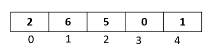
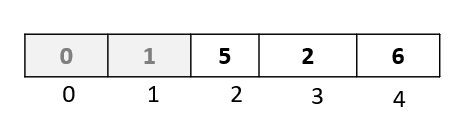
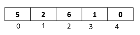
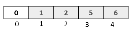
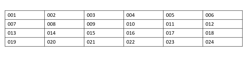
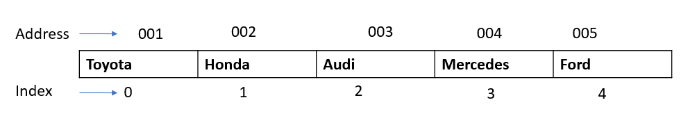
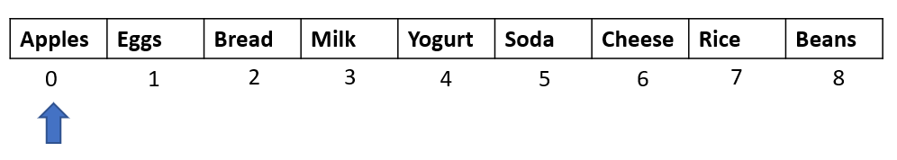
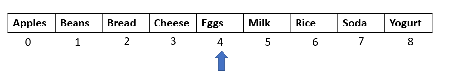
We will be sorting the following array:

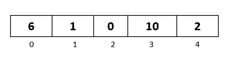
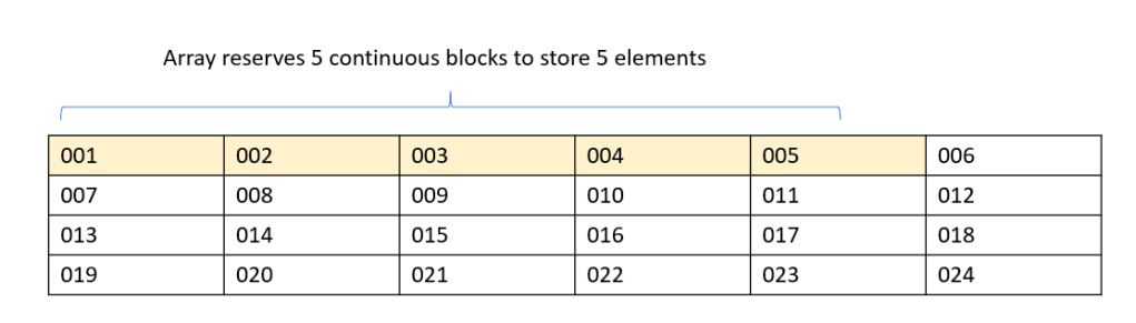
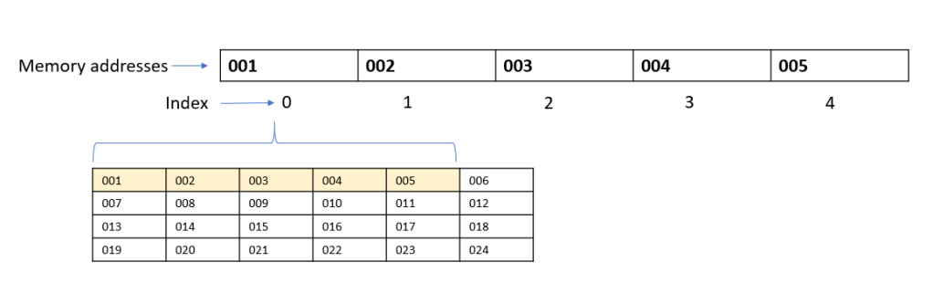
We have five elements from index 0 to index 4.

Passthrough 1

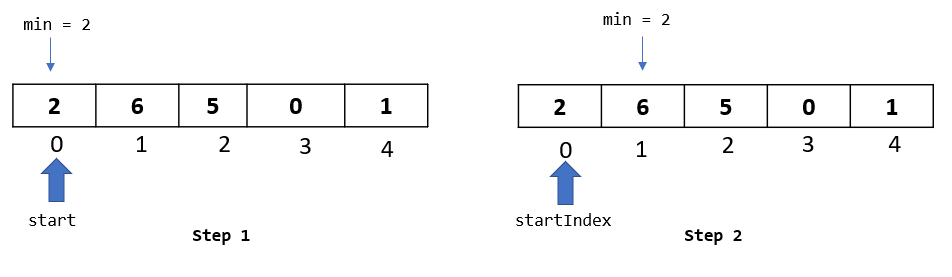
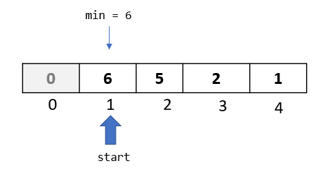
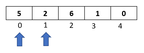
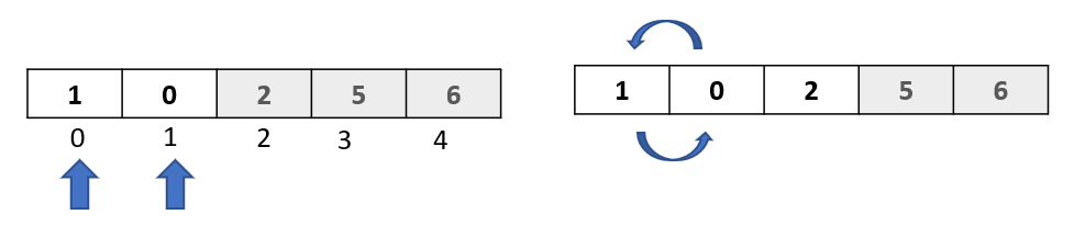
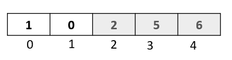
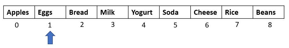
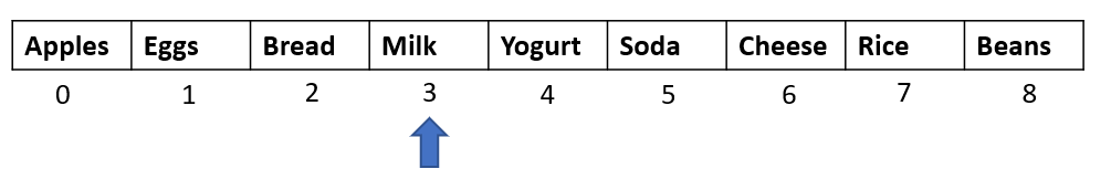
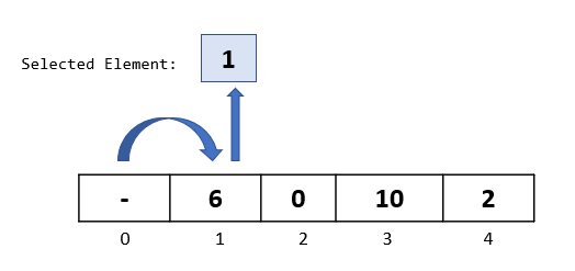
Step 1: The algorithm starts from the second element in the array, so let’s select the element at index 1.

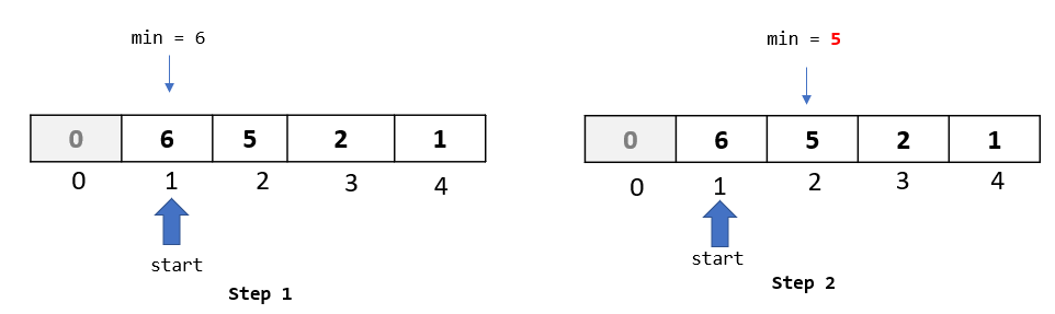
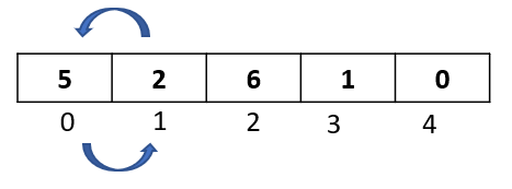
Step 2: Compare the selected element to all the elements to its left. Here we have just 1 element towards the left -> “6” at index 0. Let’s do the comparison: Is 6 greater than 1 ? Yes. Then as per the algorithm, let’s move it one spot to the right:

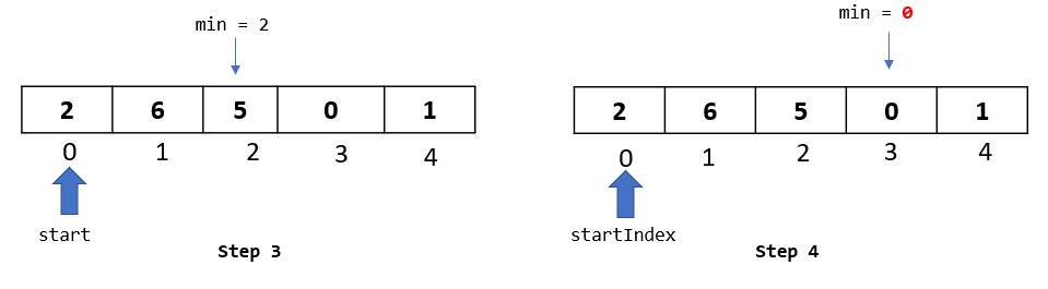
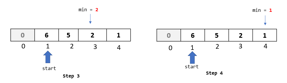
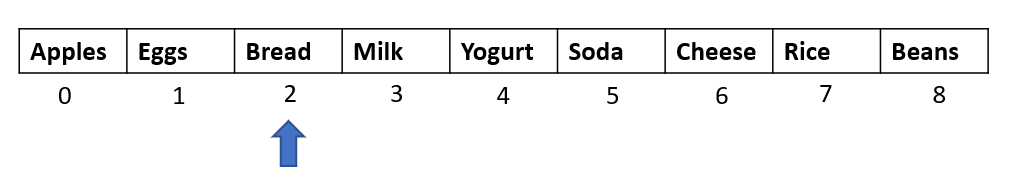
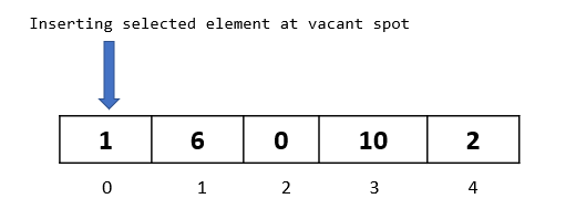
Step 3: Since we had only one element to the left of the selected element, we are done with the comparison and movements for this passthrough. Now we need to find a spot to insert our selected element.

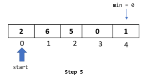
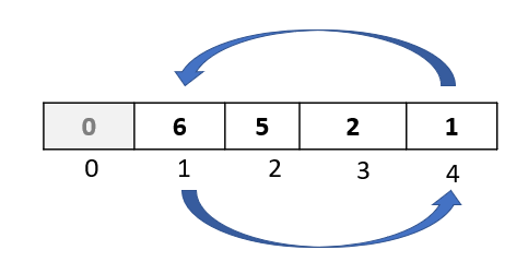
As we can see, the spot at index 0 became available, since we moved the element “6” from index 0 to index 1. So let’s insert our selected element there:

And that concludes our first passthrough.

Passthrough 2

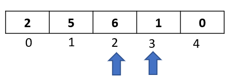
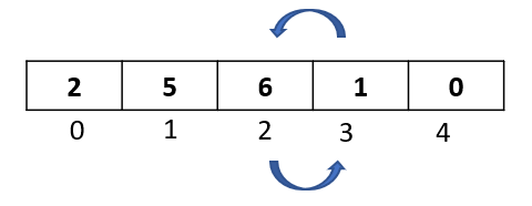
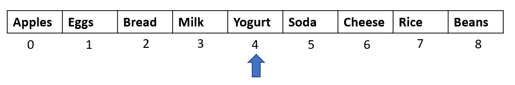
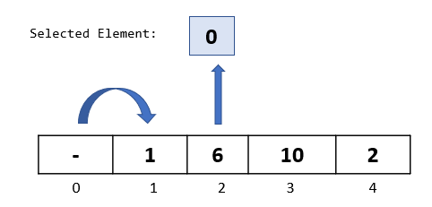
Step 1: In the first passthrough, we selected the element at index 1. In this passthrough, we will move to the next element and select the one at index 2:

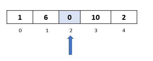
Step 2: We now begin the comparison process where we will compare the selected element to all the elements towards its left.

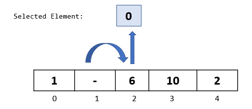
Compare selected element “0” to “6” ,the first element to its left. Since 6 is greater than 0, we will move it one step to the right

Compare selected element “0” to “1”, the second element to its left. Since 1 is greater than 0, we will move it one step to the right

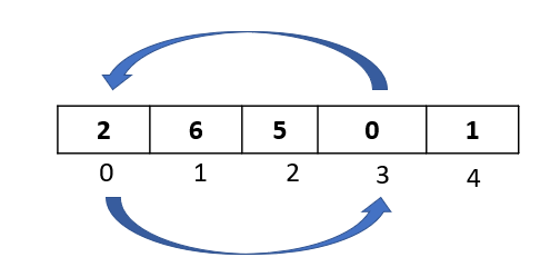
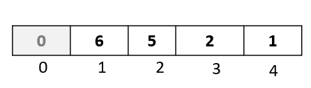
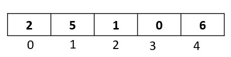
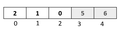
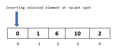
Step 3: We are done with the comparisons and movements for this passthrough. Now is the time to insert our selected element back into the array at the available vacant spot. Since we moved both the elements 1 and 6, we have a vacant spot at index 0. So let’s go ahead and insert our selected element there

Passthrough 3

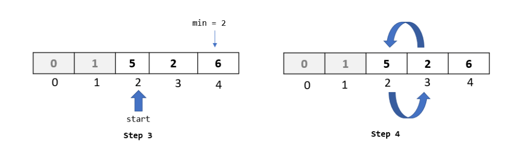
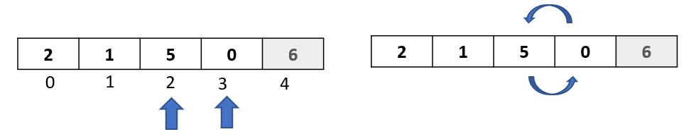
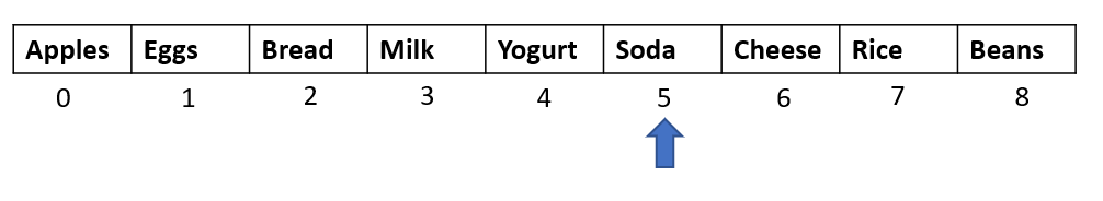
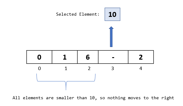
Step 1: Now that we have got a hang of the algorithm , we know that in this passthrough we will select the element at index 3.

Step 2: Let’s begin with our comparisons. We would be comparing our selected element “10” with all the elements to its left.

We do our first comparison with element “6”. Since “6” is not greater than 10, we do not move it to the right.

Also, from our previous passthroughs, we know that all the elements that are to the left of 6 are smaller than 6 (because of all the previous steps that we did). This means that in this passthrough, we do not need to move any element to the right.

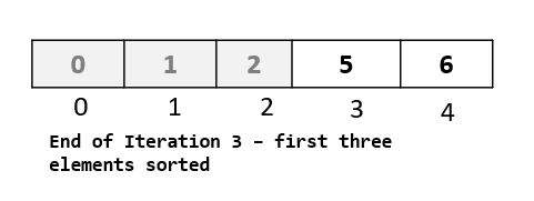
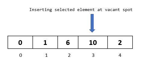
Step 3: We need to insert our selected element to an available spot in the array. Since we moved no element in the last step, the vacant spot would be the same position at which the element was before the passthrough. Hence, we put the element back at that position, and move on to the next passthrough.

Passthrough 4

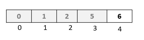
Step 1: We move to the next element in our array, and select the element at index 4. Note that this is the last element in the array, and so this will be our last passthrough

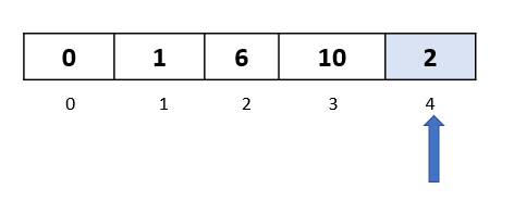
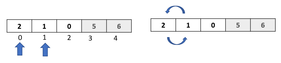
Step 2: We now begin with our comparisons. We need to compare the element “2” with all the elements to its left.

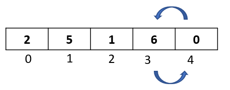
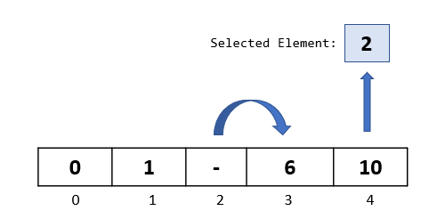
Let’s start with the element at index 3 -> “10”. Since 10 is greater than 2, we move it one step to the right.

We now compare the selected element “2” with the element at index 2. Since 6 is greater than 2, we move 6 one step to the right

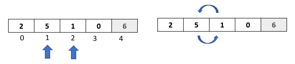
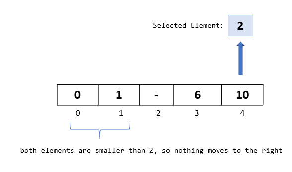
We now compare the selected element “2” with the element at index 1. Since 1 is not greater than 2, we do not move it to the right.

Also, because of our previous passthroughs and steps in the algorithm, we know for sure that all the elements towards the left of “1” would be less than “1”.

Step 3: After we have completed all the comparisons, we now need to insert our selected element back to the vacant spot in the array. Since we have the spot at index 2 vacant, we insert our selected element at index 2

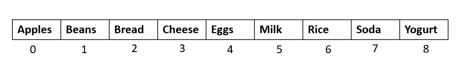
And with the end of this passthrough, we have sorted our array!

Recap

Insertion sort is a bit tricky to understand as it has a lot of steps, and it compares elements in the other direction (towards the left), as opposed to other “forward looking” algorithms that compare the elements to their right.

So let’s recap what we did once again:

  • We did 4 passthroughs for an array of 5 elements
  • In each passthrough, we selected one element
  • We compared the selected element to all the elements to its left
  • Whenever we found an element greater than the selected element, we moved that element to the right
  • At the end of all the comparisons and movements, we had one vacant spot available in the array. We inserted our selected element to that spot ending our passthrough.

And hopefully now it makes sense why it is called insertion sort!
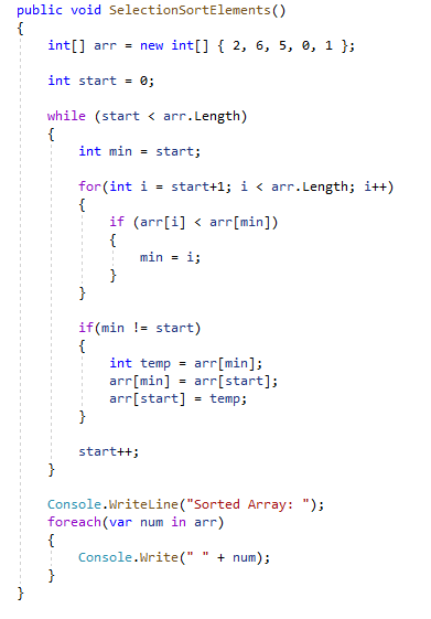
Implementation in C#

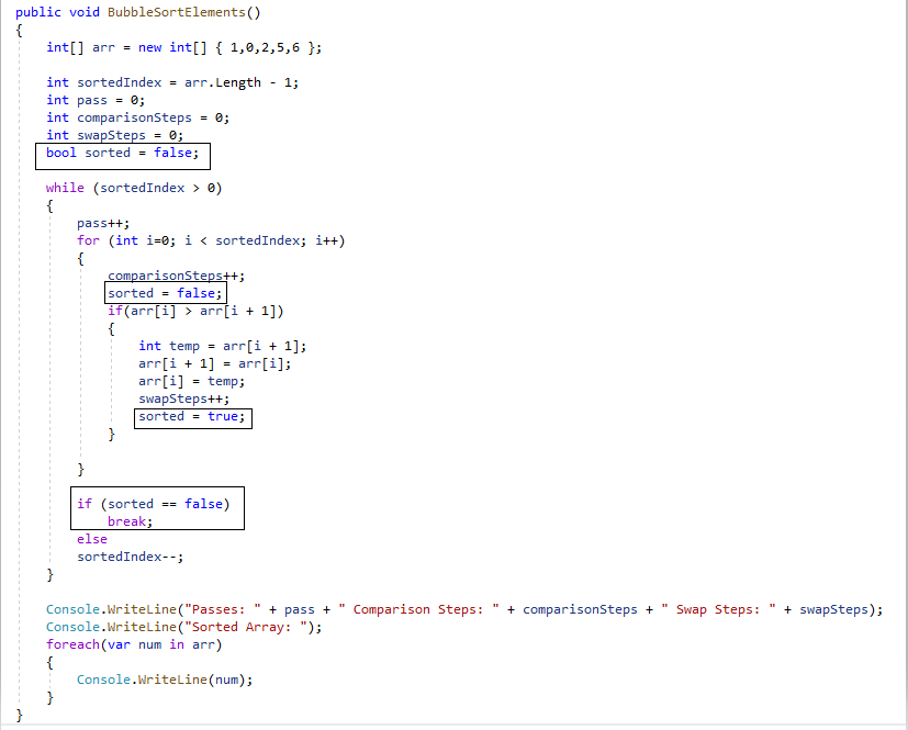
Here is an implementation of the insertion sort algorithm in C#

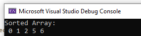
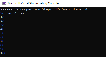
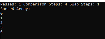
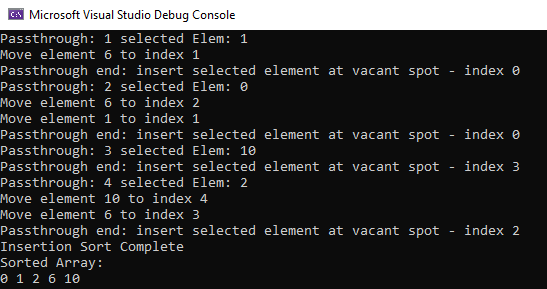
On running the above code, we get the following output:

Growth Complexity Analysis

Before jumping to mathematical terms that involve the variable “N”, let’s first try to look how many operations we performed in our algorithm.

We did the following operations on our array of 5 elements:

  1. 4 passthroughs
  2. 1 comparison and 1 movement operation in the first passthrough
  3. 2 comparison and 2 movement operations in the second passthrough
  4. 1 comparison and no movement in the third passthrough
  5. 3 comparisons and 2 movements in the fourth passthrough
  6. We also did 1 selection and 1 insertion operation in each passthrough, giving us a total of 4 selection and 4 insertion operations

This gives us a total of 4 passthrough + 7 comparisons + 5 movements + 4 selections + 4 insertions

Or a grand total of 24 operations for our array of 5 elements. Which is closer to (5) squared.

Let’s now try and derive a generalized complexity in terms of “N”.

Let’s focus on a worst case scenario – a case where all the elements in the array are in descending order.

For 1 passthrough we will do approximately: 1 selection + 1 insertion + (N-1) comparisons + (N-1) movements

And so for (N-1) passthroughs we would do approximately:

(N-1) * (1 + 1 + (N-1) + (N-1)) operations

If we ignore all the constants, we get something like:

(N) * (N)

which is equal to (N)^2 (n squared) operations

Thus we can say that the worst case complexity of an insertion sort is O(N^2) or order of N squared.

Summary

Insertion sort begins with the second element and iterates the array till the last element. In each iteration or passthrough, we select one element and compare it with the elements to its left. Whenever the elements to the left are greater than the selected element, we move them one step to the right. We then insert our selected element back to the array at the vacant spot.

This whole process would take a time complexity of O(N^2) in a worst case scenario.

feature image source: https://www.pexels.com/@digitalbuggu

Selection Sort: Implementation and Analysis

Sorting plays an important role in any computer application. When processing large amounts of data, by using efficient sorting algorithms we can bring order to our data, which streamlines our data analysis process. Today, we will dive deep into one such sorting algorithm – selection sort (for more algorithms, head over to https://getsetcode.blog/algorithms/)

Selection sort – Definition

Selection sort is one of the easier algorithms to understand. Let’s first look into how this algorithm works, then analyze the time it takes to process data, and finally understand how this efficiency changes as we pump in more data. We will also implement the algorithm in C#.

Selection sort works on the Array data structure, and a simple definition would be as follows – “For N elements in an array, loop N-1 times, and in each iteration, select the smallest element and bring it to the first index of that iteration”

Let’s jump right into an example and work our way through to understand the algorithm.

We wish to sort the following array:

As per the definition,

  1. We are going to loop 4 times (N-1 times). Let’s call 1 loop as 1 iteration of the array
  2. In every iteration, we are going to find the smallest element, and bring it to the starting position of the iteration.

In order to accomplish the above, let’s define the variable start to track the start position of every iteration, and also let’s define the variable min to track the minimum element in one iteration.

To begin, Let’s initialize start at index 0, and also min equal to the element at index 0:

Iteration 1

We now start iterating the array. Whenever we move to the next element, we check if that element is less than our min element. If yes, we assign that element to min. If not, min remains unchanged and we keep moving forward to the next element. We will do this till we reach the last element of the array:

note that start will always point to the first position of the array

We have now reached the last element of the array, and have identified the smallest element “0” at index 3.

As a last step in this iteration, we will swap the minimum element, with the element at the start position:

This will give us the following array, with the minimum element at the first position. Note that at this point we have sorted the first element. Let’s gray out the first element to highlight that it has been sorted and from the next iteration we do not need to look at this element.

Iteration 2

We were able to sort one element in the last iteration, but we have four more elements to go! Since, the element at index 0 is already sorted, we will begin this iteration from index 1. Let’s initialize our start and min variables again:

Like we did last time, we will iterate through the array, checking for the minimum element at each index, until we reach the end of the array:

We have now reached the last element of the array, and have identified the smallest element at index 4. As we did in the last iteration, we will swap this smallest element with the element at the start position of this iteration:

After this step, we now have the first two elements in our array at correct or sorted positions:

Now that we have got a hang of the algorithm, let’s quickly do all the remaining iterations.

Iteration 3

Iteration 4

Note that in this iteration, the minimum element identified is “5”, which is at index 3, which is also the start index of this iteration. Thus, the minimum element is already at its correct position, and we do not need to swap it with any other element:

The 4th iteration was our last iteration. We sorted 4 elements in these iterations. We are just left with the last element, and since all the other elements are sorted, we can safely say that the last element is also in the correct position. This is why the selection sort runs N-1 iterations for N elements.

Quick Recap

  1. For N elements, the algorithm runs N-1 iterations
  2. For each iteration, we identify the start position and assign the min element to be equal to the element at that start position
  3. We iterate through the array till the last element. For every element we check if it is less than the min element. If yes, we replace the min element
  4. At the end of the iteration, we have identified the min element and we swap it with the element at the start position

Implementation in C#

Here’s an implementation of the algorithm in C#.

  • arr represents the array to be sorted
  • start represents the start position of the array. With every iteration, we will increment start by 1. The algorithm will run until start reaches the end of the array
  • min represents the index of the minimum element. We initialize this equal to the start position.

Let’s break the code into pieces to understand it better:

  1. We will run the algorithm until start reaches the end of the array:

2. The for loop below represents one iteration. We initialize min to be equal to the start index. We then go through each and every element starting from “start + 1” index and until the end of the array. We compare each element with the element at the “min” index. If we find a smaller element, we re-assign the min index

3. Finally, if the min index is different from the start index, we swap the elements at both these indexes to bring the smallest element to the first position:

on running the above algorithm, we get the sorted array:

Complexity Analysis

We have three primary operations in selection sort:

  1. Iterations – In our example of 5 elements, we did 4 iterations. Thus we can say that for N elements, selection sort will run N-1 iterations
  2. Swaps – At the end of every iteration, we performed one swap – the minimum element was swapped with the element at the first position
  3. Comparisons – comparison is the operation when we check if each element is smaller than the minimum element. For our first iteration, we did 4 comparisons, for the second iteration we did 3, for third iteration we did 2 comparisons and for the 4th iteration we did 1 comparison. In other words we did: (N-1) + (N-2) + (N-3) … + 1 comparisons.

For 1 iteration, we did: 1 swap + N-1 comparisons

For (N-1) iterations, we will do approximately: (N-1) * (1 swap + N-1 comparisons )

If we ignore all the constants in the above equation, we will get N * N, or N squared (N^2).

Thus, the complexity of selection sort is O(N^2).

Efficiency of Algorithm with increasing data

We derived the complexity of the algorithm as N squared. If we plug in numbers, we can see how the number of operations that the algorithm takes increases:

N = 5, N^2 = 25

N = 10, N^2 = 100

N = 15, N^2 = 225

This shows that by increasing the number of elements by 5, we are increasing the number of operations at a really fast pace. Just by going from 5 to 10 elements, we increased the number of operations by 75! When we went from 10 to 15 elements, we increased the number of operations by 125!

Thus, as the data increases, the algorithm efficiency decreases and so selection sort is not a good choice when it comes to sorting huge amounts of data.

Summary

  • Selection sort works on array data structures. It loops through the array N-1 times, and in each loop finds the smallest element. This element is swapped by the element at the first position.
  • The primary operations in this algorithm are iterations, swaps and comparisons. By calculating the number of operations, we can derive the complexity of selection sort as O(N^2)
  • As we increase input data, the number of operations done by the algorithm increases at a much faster rate, making selection sort a bad choice for large amounts of data.

Bubble Sort: Implementation and Analysis

Sorting is the lifeline of coding. We almost always want things in a natural order. An alphabetical order of a list of items is easier to comprehend. Going over your bank transaction history, ordered by date, is much better to analyze.

Today we have high-level, easy to read and write programming languages which usually have a built-in sort function. For instance, in C# you just need to call the Array.Sort() method, and C# would do the rest for you.

But understanding what is happening behind the scenes makes you a much better programmer. You can analyze how fast or slow your data is being sorted and what impact that algorithm is having on your application.

In this article we will look at the most basic sorting algorithm – Bubble sort. It has a fun name, and is easy to understand. We will first learn what bubble sort is and analyze the complexity of the algorithm. Then we will write some code in C#. We will also try to improve the performance of our code with the help of a boolean variable.

Bubble Sort – Definition

Bubble sort to sorting algorithms is like learning A-B-C-D to understand the English language! Let’s jump write into an example and learn the algorithm step by step. Consider the following array of numbers:

Start with the first two elements in the array and compare them. If the first element is greater than the second element, swap the elements.

Compare:

Swap:

Move on to the next two elements. Compare and Swap again as we did in the last step:

Compare:

Since these two elements are already sorted, we do not swap and move on to the next two elements

Compare:

Swap:

And finally compare and swap the last two elements:

Compare:

Swap:

We worked our way till the last index. And now our array looks like this:

I will pause here to point out that this is just one pass of the array. We went from index 0 to index 4, comparing and swapping along the way, and the outcome of this pass is that the highest element in the array (6) is at the last position. In other words, we have bubbled the highest element out to the last position – hence the name, bubble sort.

As you might have guessed, the algorithm does not stop here, as after the first pass, we have just brought one element to its correct position, and we still have the first four elements in wrong positions.

And so, we do another pass, but this time we go from index 0 to index 3 (as our last element has already been sorted). Let’s gray out the last element to make things clearer. Now that we have got a hang of how the comparison and swapping works, lets quickly go through the second pass:

After this pass, we have now brought the second highest element in our array to the correct position:

We are already down 2 passes, but our array is still not sorted. Let’s do another pass, but this time only till index 2, as the last two elements have been sorted:

After the third pass, our third highest element is in position:

We have one more pass to go, as the first two elements are still not sorted. This fourth pass will have only one comparison and swap operation:

and after this step, we have our sorted array:

Analysis and Complexity

Let’s stop here and note a few things that happened along the way:

  1. We had 5 elements in our array, and we were able to sort the array in 4 passes. This means that for N elements, bubble sort will walk through the array N-1 times.
  2. With every pass we are able to sort 1 element. When you look from this perspective, we can again conclude that for an array of N elements, we will need N-1 pass-throughs of the array.
  3. In pass 1, we did 4 comparisons. In pass 2, we did 3 comparisons. In pass 3, we did 2 comparisons. In pass 4, we did 1 comparison. Thus, for an array of N elements, a bubble sort will do (N-1) + (N-2) + (N-3) +……+ 1 comparisons. In our example of 5 elements, we did 4+3+2+1 = 10 comparisons.
  4. In pass 1, we did 3 swaps, In pass 2, we did 2 swaps, in pass 3, we did 1 swap and in pass 4 we did 1 swap again. This sums up to 3+2+1+1 = 7 swaps.
  5. To summarize, to sort our array of 5 elements, we did 4 passes + 10 comparisons + 7 swaps = or a total of 21 steps or operations. We can also say that the total number of steps are close to (5)^2 (5 squared).
  6. The worst case scenario would be when we have the array sorted in reverse order (descending). In that case we will have a swap with every comparison. In our above example, if all the elements were in descending order, then to sort our array we would have done 4 passes + 10 comparisons + 10 Swaps for a total of 24 operations. (again almost equal to 5^2)

If you followed and understood all the 6 steps that we just did, then you just solved the complexity of a bubble sort! For an array with N elements, a bubble sort will take close to N^2 steps to fully sort the array. In other words, the complexity of a bubble sort is O(N^2) or order of N squared. That means if we have an array of 6 elements, a bubble sort will take close to 36 steps, for 10 elements 100 steps, for 20 elements 400 steps. As you might have guessed, bubble sort is not a great choice when we have huge amounts of data. But by learning bubble sort, and by understanding why it gets in-efficient as the data increases, we can develop better and faster algorithms!

Implementation

Following is an implementation of bubble sort in C#:

  • sortedIndex is initialized to point to the last element of the array. With every pass we will reduce the sortedIndex by 1
  • Pass variable will track the number of passes of the array we do to fully sort the array
  • ComparisonSteps variable will track the number of comparisons we do
  • SwapSteps variable will track the number of swaps we do
  • While (sortedIndex > 0) represents each pass of the array.
  • The for loop covers all the comparisons and swaps in one pass

As you can see, we have initialized an array of 10 elements, and the array is in descending order. This case represents a worst case scenario. On running the above code, we get the following:

The algorithm takes 9 passes, 45 comparison steps and 45 swap steps to give a total of 99 steps, which is close to 10 squared. Thus giving a great example of the complexity of the algorithm.

A slightly better implementation

The implementation that we did earlier will take N-1 passes and compare every two elements along the way. Now consider a case when some elements of the array are already sorted. For example:

Here, the last three elements are already sorted, but according to the algorithm we will still need to compare all the elements.

We can slightly improve the implementation of our algorithm to first check if we already have a sorted array. In a pass, we will track if there were any swaps made. If not, it implies that we already have all the elements sorted, and we no longer need to pass through the entire array again.

We will declare a boolean variable “sorted” which will be set to false. During 1 pass, if we make a swap, we set the variable to true. Now, if we complete the pass, but we did not do any swap (because all elements were already sorted), the boolean variable “sorted” will still be set to false. This will indicate that the array has been sorted, and we can safely end the algorithm.

Our modified code will be as follows:

On running the above code on the array [1,0,2,5,6], we get the following output:

Note that we took only 1 pass and 1 swap step!! All because we checked along the way if the rest of the array is sorted, and exited the while loop when we no longer needed to go through each and every element.

Summary

In this article we did a deep dive to understand the bubble sort algorithm. It is a simple sorting algorithm which compares each and every element in an array, moving the greater element to the right with every pass.

The complexity of bubble sort is O(N^2), and we did an in-depth analysis and implemented code to understand that. Bubble sort might not be a good algorithm to sort large amounts of data.

Feature Image: https://www.pexels.com/@padrinan

The World Of Arrays

Brands of cars. Debit card transactions in a day. A shopping list. All these represent a list or collection of things that can be grouped into a particular category or type.

TypeValue
Car Brands“Honda”, “Toyota”, “Hyundai”, “Ford”, “Audi”
Debit Card Transactions“$25”, “$45.67”, “$140”, “$10”
Shopping List“Jeans”, “Groceries”, “Books”

These all types can also form the data that a computer program works upon. For instance, whenever you do a self-checkout at Walmart, the software that calculates the total due amount would first need the details of the items that you bought from the store. But how does a computer store and process such a list of items?

Here is where data structures come into play, and when it comes to a collection of items, Array is a simple and powerful data structure that stands out.

Definition of Arrays

Array is a type of data structure that stores a collection of items at contiguous memory locations. What does contiguous memory locations mean? Well, think of the computer memory as a collection of blocks, where each block has its unique address (001, 002, 003…..and so on)

Imagining the computer memory as blocks with unique addresses

Each block can be considered as a small storage unit which can hold one element. An array of 5 elements will occupy 5 consecutive blocks in the memory to store its data.

Each memory location is referenced by an index. The first position would be index 0 (and will also be the address of the array). The subsequent indexes would be 1,2,3 and so on.

And now if we want to store the values of car brands in our array, the computer will store them as follows:

Delcaring and initializing arrays

An array is usually declared in a programming language as follows:

//This is C# syntax
//Other programming languages may declare arrays a bit differently

int[] arr = new int[5] // an array to store 5 integers

string[] cars = new string[5] // an array to store 5 car brands

The square brackets [] indicates the compiler that we are declaring an array, and the number inside the square brackets [5] indicates that the array would contain five elements. We need to specify the number of elements in advance, so that the array can reserve the appropriate block of memory to store the elements. (There are collections like dynamic arrays and Array lists which do not require us to specify the number of elements in advance, but these topics are not in the scope of this article)

By using indexes, we can add data to the array:

cars[0] = "Toyota" //adding Toyota to position 1
cars[1] = "Honda"
cars[2] = "Audi"
cars[3] = "Mercedes"
cars[4] = "Ford"

Reading From an Array

We can read data from the array using indexes as well

string myCar = cars[1] //read the car at index 1 or position 2 in the array

Reading from arrays is a fast operation. The computer knows the address of the array, and if we know the position of the value to be read, the computer can do a quick calculation of (address + position) and jump to that address. This is the power of storing items at contiguous locations.

In laymen terms, to read an element from an array takes only one step -> the computer calculating the address of the desired element and reading it.

In computing terms, the read operation of an array would always take constant time, which can be represented as O(1) or order of 1.

Inserting elements into an Array

Data can be inserted into an array, again by using indexes.  The easiest way to add data to the array is at the end of the array.

In the above example, we can add an element at index 5 as follows:

cars[5] = "Hyundai"

We can also insert data in the middle and beginning of an array. But this operation is a bit inefficient as we need to shift data in the array to accommodate for the newly added element. For example, if we have to insert “Kia” at index 2, then we would need to move Audi to index 3, Mercedes to index 4 and so on:

The worst case would be to enter data in the beginning of the array, as we would have to move all values one index to the right:

In laymen terms, we can say that for an array of “n” elements, the worst case scenario would be to insert an element in the beginning, which would require us to shift elements “n” times before the new element can be inserted.

In formal or computing terms, this operation would take “n” time in the worst case scenario and this complexity can be represented as O(n) or order of n.

Deleting from an Array

Deletion would be similar to insertion. Deleting an element from the end of the array would be the easiest. But, if we wish to delete an element from the beginning or middle of the array, then we need to shift all the remaining elements one position to the left.

Deleting from the middle. The elements “Mercedes” and “Ford” need to be moved one position to the left
Deleting from the beginning would require all the other elements to shift one position to the left

Like insertion operation, the worst case scenario for deletion would be the case when we want to delete an element from the beginning and we will have to shift all elements one index to the left. Thus, the complexity of the deletion operation is O(n) as well.

Searching an Array

If we want to search an element in an array (that is, we do not know the index of the element before hand), then we would need to traverse the array until we find that element. The best case scenario would be that the first element in the array is the element that we are looking for. The worst case would be the case where the element is in the end. In such a case we will have to traverse the entire array to get to the last element. Again, the complexity of searching an element in the worst case would be O(n).

Another worst case scenario would be that the element that you wish to search does not exist in the array at all. That would also lead to a full traversal of the array leading to a complexity of O(n).

Summary

  • Arrays are data structures which store a collection of items in contiguous memory locations
  • Each element in an array is assigned an index. The first element will start from index 0
  • Elements can be added and removed from the array using indexes
  • Reading operation takes constant time O(1) and this is one of the strengths of an array
  • Insertion, deletion and search operations take O(n) time in the worst case

A Quick Introduction To Data Structures

Suppose you went to a grocery store and bought two items, let’s say a can of beans and a small packet of rice. You went to the checkout counter, paid for the can of beans and rice, and politely refused to take a bag as these are just two items which you can carry one in each hand and walk to your car. Great!

Now imagine you went to the grocery store and bought eggs, bread, apples, spinach, lettuce, carrots, pasta sauce, pasta….. And you go to the checkout counter. Now you definitely need a bag! As you cannot carry all these items with your two hands, even if it is a short walk to your car.

Computer systems are the same!  Our computer programs work on data and logic. For example, in the program to calculate the sum of the numbers 1 and 2, the data would be the numbers 1 and 2 and the logic would be the addition operation. In such small programs, we do not essentially need a data structure. 

//data - Just two numbers, we can manage without a data structure
int one = 1;
int two = 2;

//call the logic
Sum(one, two)

//the logic
int sum(int a, int b){
 return (a+b);
}

But we seldom write such small programs in the real world. Consider a similar program which calculates the sum of all the numbers between 1 and 100. It would get really messy to handle 100 numbers if we start assigning a variable each to every number.

//data of a hundred numbers
int one = 1;
int two = 2;
........
int hundred = 100;

//calling the sum logic 
//since the sum method accepts only two  numbers
// we need to call the method again, and again, and again
int result = sum(one, two)
result = sum(three, result)
result = sum(four, result)
... 
//and so on

Do we really need over a 100 variables just to calculate a sum of numbers?

Well, we can also use a for loop to make this a bit cleaner, since we know the range of numbers we are working on (1-100)

int sum = 0;
For(int i = 1; i <= 100; i++){
 sum = sum + i;
}

But, the input numbers would not always be in the form of a “range” which can be represented by the index variable (i) of the for loop. For example, the input numbers could be 1, 200, 99, 450, 77 and so on.

This is where data structures come into play. Just like bags in a grocery store which help organize your groceries, data structures are nothing but storage units which the computer uses to organize the data in its memory.

Let’s go back to the grocery bag example.

Would you put loose eggs into a bag? No, they will break! That’s why the eggs are packed in a crate – neatly organized so that they may not break. Similarly, when you start putting groceries in a bag, you will not put tomatoes first and then a bottle of pasta sauce on top of it to avoid the tomatoes from squishing. Thus, when we start putting stuff in the bag, we would sub-consciously be taking care of the following:

  1. Every item is inserted in the bag properly so that nothing breaks
  2. Every item can be retrieved from the bag in proper condition
  3. Every item can be easily searched in the bag, without damaging the bag or other items
  4. Every item can be removed from the bag, without damaging the bag or other items

That is exactly how the computer works with data structures. Each “structure” stores data in such a way so that the basic operations of insertion, retrieval, deletion and search can be done easily without breaking the data structure or affecting the data.

Different Data structures store data differently to cater to different operations that can be performed on the data. Some data structures support easy insertion , while others provide fast search. Following are some common data structures that you would encounter in your coding life:

Arrays: A structure which stores  a series of data elements in contiguous locations in memory for easy retrieval

Linked Lists: Like arrays, store a series of data elements. Unlike arrays, does not store in contiguous locations. Data is stored in nodes. Each node has a pointer to point to the memory location of the next node (which has the next data). This allows for better insertion and deletion operations as compared to arrays.

Maps / Dictionaries: Store data as key-value pairs to search data efficiently

Trees/ Graphs: Like linked lists, Trees store data in nodes. Each node is structured in a way that it can have a parent and children. Graphs are similar to trees in the sense that all nodes are connected to form a kind of network. These are advanced data structures and provide the means to solve complex algorithms.

Thus we can see that different structures organize data differently providing their own advantages. This was a super fast introduction to the world of data structures, to give you an understanding of where data structures come from (without intimidating you!).

To summarize:

  • Data structures are nothing but different ways in which the computer organizes the data being used in a program
  • Different operations that can be performed on data structures are: insertion, deletion, retrieval and search of data elements
  • There are many data structures which are being used in real world programs. They all organize data differently, with different strengths when it comes to the different operations
  • Arrays, linked lists, maps, dictionaries, trees and graphs are some examples of data structures.

In my upcoming posts, we will do a deep dive into the various data structures and start solving real world problems using those data structures.

Let’s uncomplicate coding!

K.

Analyzing Linear and Binary Search Algorithms

Search can be considered as one of the most essential features that a software product can have for a good user experience. For instance, whenever we log onto amazon, we can directly go to the search bar and enter the product that we wish to buy, rather than going through all the products one by one!

Search algorithms can get really complex as the amount of data increases, and the key to writing efficient algorithms would be to first understand the basics. Today we will look into two simple search algorithms that work on the Array data structure. This will give you a perspective on how search operation is performed and the implications on efficiency when input data is increased.

Linear Search

As the name suggests, linear search goes over all the items in the array, one by one, until we find the desired element.

Let’s say we have the following array which stores a list of products added to an online grocery shopping cart:

At checkout, we decide to remove Soda from the list. Now in order to do that, we would first need to find the exact location of the item “soda” in our list.

A linear search would proceed as follows:

Step 1: Start from index 0. Is the item “Soda” ?

Nope the item is not Soda. Proceed to the next element

Step 2: Is the item at index 1 “Soda”?

Nope. Proceed to the next element

Step 3: Is the item at index 2 “Soda”?

Nope. Proceed to the next element

Step 4: Is the item at index 3 “Soda” ?

Nope. Proceed to the next element

Step 5: Is the item at index 4 “Soda”?

Nope. Proceed to the next element

Step 6: Is the item at index 5 “Soda”?

Yes! Finally! Phew!

The item soda was found at index 5 (or position 6) in the array by our linear search algorithm. In order to find an item at the 6th position, the algorithm took 6 steps. If Soda was present at position 7, then the algorithm would have taken 7 steps. Thus, we can say that Linear search will take n steps for finding an element at nth position. In other words, the complexity of the algorithm is O(n) or order of n.

Implementation in C#

Following is an implementation of the linear search algorithm in C#:

 public void LinearSearchProduct()
        {
            string[] cart = new string[] { "Apples", "Eggs", "Bread", 
                             "Milk", "Yogurt", "Soda", "Cheese", "Rice", 
                             "Beans" };
            string item = "Soda";
            bool found = false;

            //For loop will go over each element of the array
            for(int i=0; i < cart.Length; i++)
            {
                if(cart[i] == item)
                {
                    found = true;
                    Console.WriteLine("Product found at index: " + i);
                    break;
                }
            }

            if(found == false)
            {
                Console.WriteLine("Product not found");
            }
        }

Growth Analysis

In our example, we just had an array of nine elements. Imagine if the array contains thousands of elements. Even worse, imagine if the item that we are interested in is at the last position in the array! Since the linear search algorithm would need to go over the entire array, it would probably not be a great option to use when we have large amounts of data.

As we can see in the table below, for every new element added to the array, Linear search would need one additional step to find an item, following a growth complexity of O(n):

Number of Elements in ArrayMaximum Number of Steps Taken by Linear Search
55
66
77
88
99

Binary Search

Binary search is a much faster algorithm than linear search. The only caveat is that Binary search expects the data in our array to be sorted. In other words, the binary search algorithm works on ordered arrays. Once we understand how the algorithm works, this will make much more sense.

The algorithm works by eliminating or ignoring half of the elements of the array with every step until we find the desired element.

First, it starts by looking at the middle element of the array. If the item to be searched is equal to the middle element, we get our result.

Else, it checks if the item to be searched is less than or greater than the middle element.

If the item is less than the middle element, then it considers the first half of the array for the next step and ignores the second half.

If the item is greater than the middle element, then it considers the second half of the array and ignores the first half.

Whichever half it chooses, it repeats all the above steps again by checking the middle element and comparing it with the item to be searched.

We do this until we get the desired element.

Let’s go back to our example to visually see how it works:

This image has an empty alt attribute; its file name is image-13.png

We want to search for the item “Soda” in the above array.

First step would be to sort this array following natural ordering (ascending order or Alphabetical in case of strings). So the following would be our input array.

Step 1: Find the middle element of the above array. If the length of the array is n, then the middle element would be n/2 if n is even, and (n+1)/2, if n is odd.

Here, length of array is 9. so our middle element would be at position (9+1)/2 = 5. (This would be index 4, since arrays start from index 0)

Does the middle element = “Soda” ? Nope.

Is “Soda” less than or greater than the middle element? Greater than (Alphabetically Soda comes after Eggs)

Step 2: Select second half of the array and find the new middle element:

length of this new array is 4, so the middle element would be at the second position (4/2) – here index 6

Does the middle element = “Soda” ? Nope.

Is “Soda” less than or greater than the middle element? Greater than (Alphabetically Soda comes after Rice)

Step 3: Select the second half of the array and find the new middle element:

length of this new array is 2, so the middle element would be at the first position (2/2) – here index 7.

Does the middle element = “Soda”? Yes! Return element.

Thus, we can see that the binary search algorithm took only 3 steps to find the desired item.

Growth Analysis

One thing to note is that with every step, the number of elements that we are looking into reduce by half. Let’s look at this from another perspective, that is, for how many new elements would binary search take an additional step?

Number of Elements in ArrayNumber of steps taken by binary searchLog representation (to the base 2)
21Log(2) = 1
42Log(4) = 2
83Log(8) = 3
164Log(16) = 4

Thus we can see that whenever the elements in the array double, the binary search would take 1 additional step to find the item. This is how the time complexity grows for binary search. Since this growth can be represented in log terms, the complexity of binary search is O(logn) or order of log(n).

Implementation

The implementation of binary search in C# is as follows:

        public void BinarySearchProduct()
        {
            string[] cart = new string[] { "Apples", "Eggs", "Bread", 
                            "Milk", "Yogurt", "Soda", "Cheese", "Rice", 
                             "Beans" };
            string item = "Soda";
            bool found = false;

            //we need to sort cart to implement binary search
            Array.Sort(cart);

            int start = 0;
            int end = cart.Length - 1;

            while(start <= end)
            {
                int len = end - start + 1;
                int mid = start + (len / 2);

                if (item == cart[mid])
                {
                    Console.WriteLine("Element found at index: " + mid);
                    found = true;
                    break;
                }
                else if (item.CompareTo(cart[mid]) > 0)
                {
                    start = mid + 1;
                }
                else
                {
                    end = mid - 1;
                }
            }

            if(found == false)
            {
                Console.WriteLine("Element not found in array");
            }


Summary

  1. Linear Search iterates over the entire array, one element at a time, until the desired item is found
  2. Time complexity of Linear search is O(n)
  3. Binary Search works on a sorted array
  4. Binary Search eliminates half of the elements with every step, making the search faster.
  5. Time complexity of Binary Search is O(logn)

Feature image source: https://www.pexels.com/@pixabay